
Overview
Modern machine learning can be distilled down to a couple of techniques that can be applied to a wide variety situations. Recent studies have shown that the majority of datasets can be modeled with just 2 methods:
Ensembles of decision trees like random forests and gradient boosting machines which can be used for structured data.
Multi-layered neural networks with Stochastic Gradient Descent (SGD), mainly for unstructured data like audio, vision and natural language.
Machine learning problems can fall into 2 groups. Regression models (called Regressors) are used to predict continuous variables like the price of a product. On the other hand Classification models (called Classifiers) are used to predict categories of things like images of cats and dogs. Logistic regression is a method of clasification where the model outputs the probability of the target variable belonging to a certain class.
Evaluation Functions
Before diving into building a machine learning model, you need a way to measure how well it predicts. This is called evaluation functions and there are several:
Root Mean Square Error (RMSE)
$$
RMSE = \sqrt{ {\frac{1}{N}\sum_{i=1}^N(actual_i - prediction_i)^2}}
$$
Root Mean Square Log Error (RMSLE)
$$
RMSLE = \sqrt{ {\frac{1}{N}\sum_{i=1}^N(\log(actual_i) - \log(prediction_i))^2}}
$$
Coefficient of Determination ($r^2$)
It is a ratio of how good the model is vs a naive mean model.. Valid values include $-\infty \lt r^2 \le 1$, where 1 indicates a perfect prediction. A Negative value means the prediction is worse than predicting the mean value.
Out-of-Bag Score (OOB)
With random forests each tree is built from a different subset of the training data (Bagging). Out-of-bag score takes advantage of this by calculating the error for a given row by only using the trees where that record was not used to train the tree. It can be useful if you don't have enough data for a validation set. Because OOB only uses a subset of the trees to calculate the error, it will always be slightly worse than using a validation set that can use the entire forest to calculate the error.
How is a Random Forest Created
A random forest consists of a collection of decision trees (also called estimators). Each decision tree is built up from a different subset of the training data. During training the tree will run through the data to determine the best possible split point. The process repeats recursively for the remaining subset of records on both sides of the split until no more splits are possible.
How a split point is chosen.
There are several ways to determine the best split point. One way is trying every possible split point for every feature until you find the point with the lowest weighted avg mean squared error (MSE * number of samples in split). In other words, which split point has the best mean squared error. Another way to calculate the score is to find a split where both groups have the lowest weighted average standard deviation.
Bootstrapping
In scikit-learn each decision tree is bootstrapped with replacement, which means it is built up of a subset of the training data but of the same size as the training set (Some records are repeated). To use only a subset of the data without replacement can be achieved through set_rf_samples provided by fastai.
How is a prediction made
A given record will be passed through every decision tree in the forest until the appropriate leaf node for that record is found. The final prediction is the mean of the predictions made by every tree.
Data Preparation
Random Forests need numbers to train on, the fastai python library provides some utility functions that can be used to prepare a raw dataset.
Dates can be expanded into year, month, day, day of week and many others using the add_datepart.
Strings can be turned into panda category data type using train_cats. A category data type contains a alphabetized list of all the unique values for the given string column. The codes attribute on the category data type contains the index of the category that applies to the given record.
Finally proc_df can be used to split out the dependent variable and turn the data frame into an entirely numeric one. This is achieved by replacing the category columns with the codes attribute of the category datatype. In other words it turns a column of strings into a column integers representing the index to the list of unique categories. Missing values use -1. It also replaces missing values with the mean and adds a boolean column to the data frame with the name *$feature_*na to indicate that the given record had a missing value.
One Hot Encoding (Dummy Variables)
Normally a categorical variable like 'High', 'Unkown', 'Medium' and 'Low' will get converted to an integer that represents each category (0,1,2,3). Say for argument sake that only 'Unknown' is important in the prediction. The tree will have to split twice to reach that conclusion, once on for greater than 0 and then again for less than 2. One Hot Encoding creates a new feature with a boolean value for each category, is_high, is_unknown, is_low etc. Now the tree can split just once for each of these conditions to determine if that category is really matters.
The fastai library supports this trough proc_df, passing in max_n_cat=7 means that any categorical variable with less that 7 categories ( has a cardinality of < 7 ) will be turned into one hot encoding. This may also change the feature importance, can be useful to understand the data better. One hot encoding will create feature columns of the form feature_level.
Splitting up the data
Typically data will be broken down into 3 sets, training set, validation set and the test set. The training set is used to train the model and the validation set can be used to see how the model performs against data it has not seen before. With the validation set the dependent variable is available, thus the error of the prediction can be calculated.
The test set typically does not contain the dependent variable and is used to see how the model will perform under real circumstances. Test sets should not be used in the training process, but can be used to calibrate the validation set. The ideal validation set will provide scores that closely match that of the test set.
How to pick a validation set
Randomly picking records for the validation set is a good strategy unless there is some temporal factor. If you are predicting future sale prices then recent data is more accurate. A better approach may be to cut most recent data out for the validation set and train on the date up to before the start of the validation set, this will more closely simulate the situation in production.
One technique to figure out whether there is a temporal factor splitting the test and training is to use a random forest to try and predict if a record is in the test or training set. This can be achieved by combining both training and test set into a single data frame but adding a is_test feature to the data frame indicating whether the records is from the test set or not. At this point the normal process can be followed, split out a training & validation set then train a model on the training set to predict is_test. If the model has a high accuracy score, feature importance will highlight biggest contributers to that accuracy. If any of those are temporal in nature then its a good indicator that the test set was not random.
Tweaking With Hyper Parameters
There are a few parameters that change how the forest is built which can improve the score and performance of the model.
Subsampling
By default the RandomForestRegressor will use a different subset of the training data for every tree but of the same size as the training data (records will be duplicated), this is called bagging.
The aim of bagging is that each estimator is as accurate as possible, but between the estimators the correlation is as low as possible so that when you average out the values you end up with something that generalizes.
Not directly supported by scikit-learn but fastai provides set_rf_samples to change how many records are used for subsampling. A tree built with 20k records will have $log_2{(20k)}$ levels and 20K leaf nodes. Less nodes means the tree is smaller and faster but also less rich in what it can predict. The effect of this is that the tree will overfit less but also be less accurate in its prediction.
Minimum Leaf Samples
Changes the amount of records in the leaf node. Every time you double the amount of records in a leaf node you remove 1 level from the tree
($ log_2{(n)} - 1$). The effect of this is that the estimator will be less accurate but also less correlated.
Maximum Features
Changes the number of random features used to calculate the best split at any given node. Using all the features every time will produce trees with less variety in the forest, since all of them will first split on the most predictive feature. Randomizing the features to calculate the split will reduce this effect and produce trees that will be less accurate but also less correlated.
Tree Interpretation
Confidence Based on Tree Variance
Calculated by measuring the standard deviation between the predictions of every tree for a given record. Common records that the tree has had many examples to learn from would have a low deviation, and therefore a high confidence in the prediction. This can be used for 2 things:
- Provide a numerical value for how confident the tree is in a prediction for a given row.
- Analyzing the confidence when grouping by feature may yield insight into which features the model is less confident in predicting on.
Feature Importance
A technique to discover the most predictive features of the data that will work with any model.
Start by building a model and measuring the RMSE (or whichever evaluation metric you are interested in). Now, for every feature, randomly shuffle that column keeping all the other columns intact, effectively destroying the relationship between that feature and the rest. Measure RMSE again and note how much worse the model performed, the difference between the new RMSE and the original represents importance of that feature.
Once this has been done for every feature, the importance can be ranked based on size to determine the most important features. Using only the important features will simplify the model without sacrificing too much in accuracy.
Redundant Features
Another technique that can be applied after removing inconsequential features, is to remove features with similar meaning. This can be achieved by plotting the rank correlation of the features and removing one from every group where they are considered similar. Keep an eye on the evaluation function (RMSE, $r^2$, OOB...) to make sure removing the feature had the desired effect.
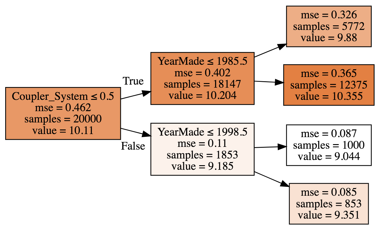
An example of a rank correlation plot from kaggle's house price prediction problem:
![]()
In the given example GarageYrBuilt and YearBuilt are in the same position in the tree and of similar importance, hence one can potentially be removed.
Partial Dependence
It is a technique that uses the random forest to analyze and better understand the data by looking at the relationship between a feature and the dependent variable. The calculation is similar to feature importance, but instead of shuffling the column, it is replaced by a constant value before running predictions against a pre-trained model. The process is repeated for every value in the range of values for that column and plotting the prediction every time.
In other words, all else being equal, what is the relationship between the given feature and the dependent variable.
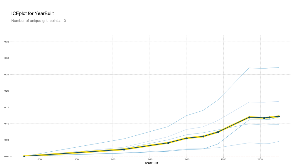
Below is an example of partial dependence plot of YearBuilt on the SalePrice for the house prices kaggle competition. Each blue line represent the SalePrice for a single record accross the range of values for YearBuilt, while the black line shows the average.
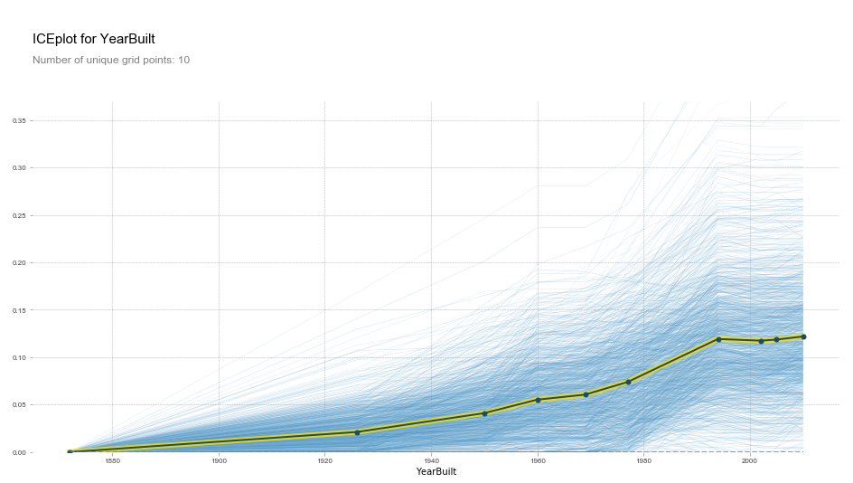
Clustering the data shows the most common relationships between YearBuilt and SalePrice.
Tree Interpreter
Can be thought of as feature importance for a singe record. For example with hospital readmission, this could explain which features will contribute most to the likelihood of readmission of a single patient. The technique starts with the bias (mean for the entire tree) then proceeds to calculate the difference between the current and previous value at every split point, that represents impact of the given feature. Waterfall charts is a good way to visualize the impact of every feature on the final prediction for a single record.
Terminology
Dependent variable - Usually what you are trying to predict, it depends on other variables (sometimes called features).
Estimator - Each tree in a random forest is called an estimator.
Features - The columns of a dataset represent the features, its all the variables that can be used to predict the dependent variable.
Bagging - Using a different set of records to train every tree in the forest.